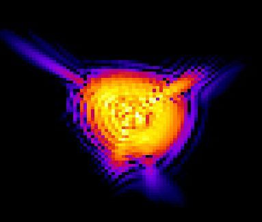
The PSF-Simulator is a small tool with which you can create three-dimensional point spreading functions and export them for further processing. In particular, aberrations up to 4th order can be taken into account by entering the Zernike terms, so that a quick estimate of the appearance and imaging properties of a given optical system can be made.
The simulation is based on the light propagation in the angular spectrum, a numerical solution of the Rayleigh-Sommerfeld integral. It is based on the decomposition of complex wavefronts into plane waves, which can be mathematically expressed by a Fourier transformation.Each plane wave can then be propagated to the target plane, where the new complex wave field is created by a Fourier re-transformation. Details about the Method can be found in [1]
The program can be downloaded as a stand-alone application for Mac and Windows. If you are interested in the Matlab code, please send me an email. More informations will follow soon!
Windows:
Windows Installer: please send me an email
Mac/ Linux
Installer: please send me an email
References (PSF-Simulator)
| 1. | : Introduction to Micro- and Nanooptics. WILEY-VCH, 2012, ISBN: 9783527408917. |
Short instruction
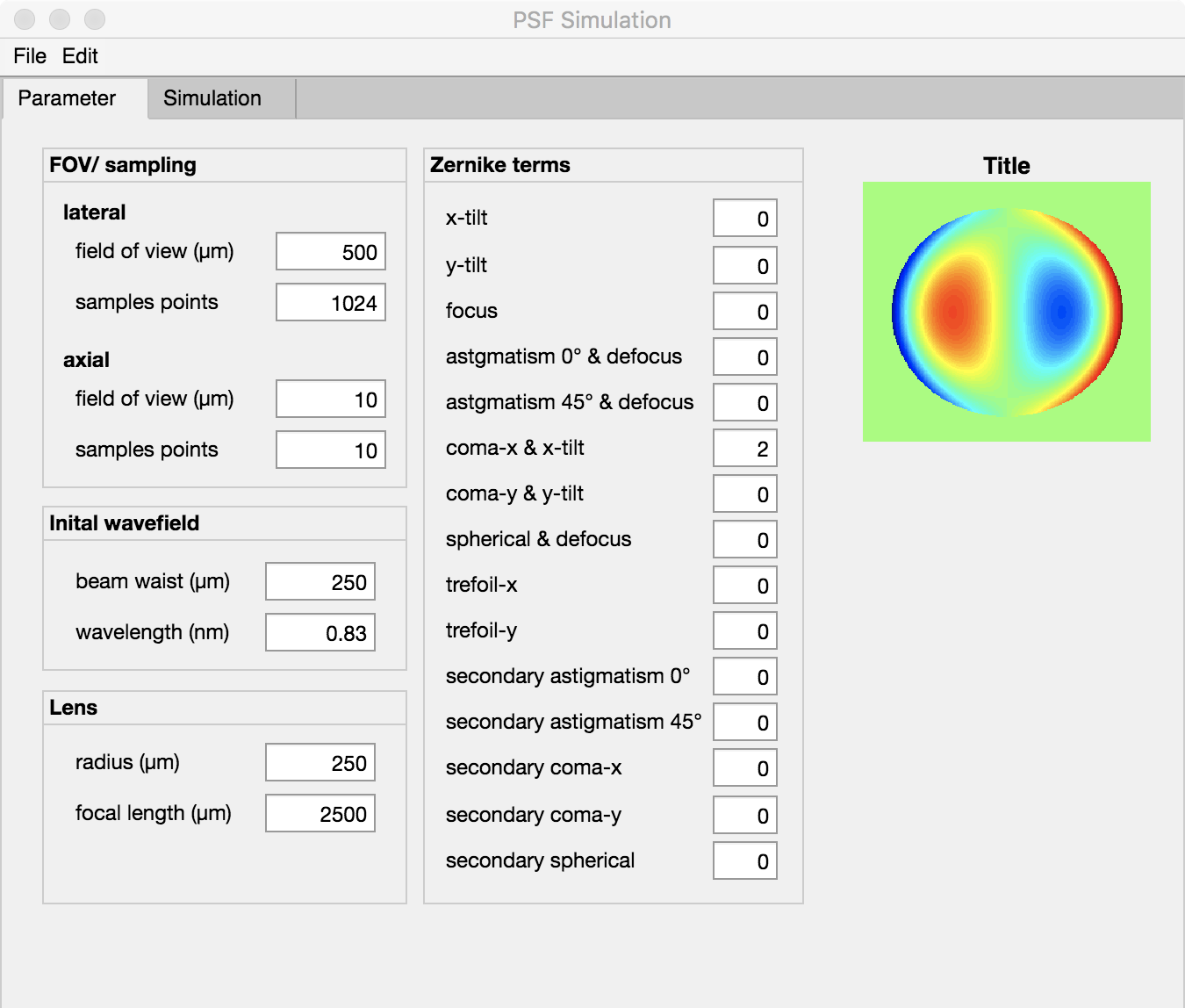
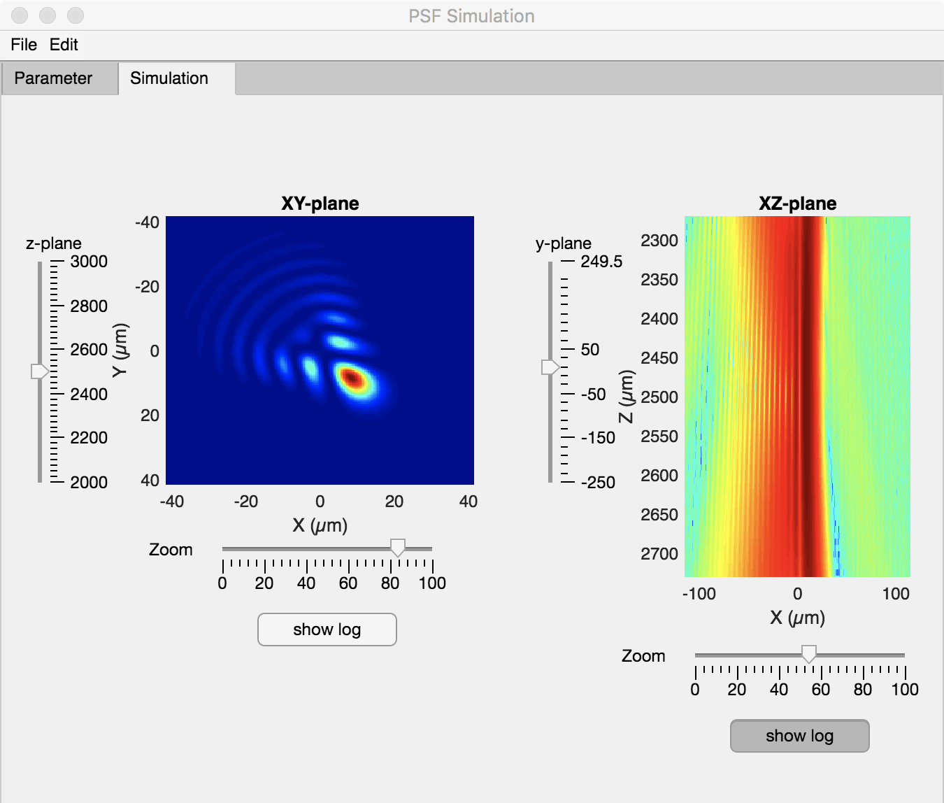
The “PSF Simulator” offers the possibility to calculate three-dimensional PSFs and then export them into a tiff stack. The geometric dimensions shall be given in um. An exception to this are the Zernike terms, which are given in wavelength as usual. The “PSF Simulator” is split into two tabs. In one the parameters are defined and in the second the simulation results are displayed.
The individual simulation parameters and controls are explained below.
The simulation can be started under Edit -> Run. The resulting three-dimensional PSF can be saved under File – Export.
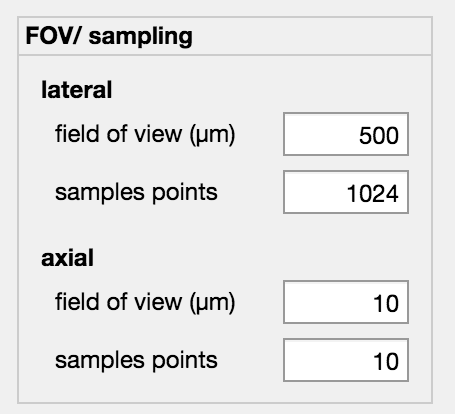
The geometric parameters for the simulation are defined in the FOV/Sampling container.
The geometric side lengths (defined as X-Y plane) of the simulation area are defined via the lateral -> field of view in um. An asymmetric definition for x and y is not possible. Another important parameter is the number of sample points. These describe the number of points in x or y direction. If Sample points = 512 then the X-Y plane is 512 x 512 pixels. The FOV and the sample points must be selected so that all room frequencies can be transmitted. This is controlled by the PSF simulator and corrected if necessary.
Under the sub-item axial the axial FOV and the number of displayed planes can be parameterized. The FOV is given in um and is semetrically around the defined focal plane. Sample Points defines the number of X-Y planes to be simulated. These are distributed equidistantly over the FOV. Sub-sampling is therefore not possible.
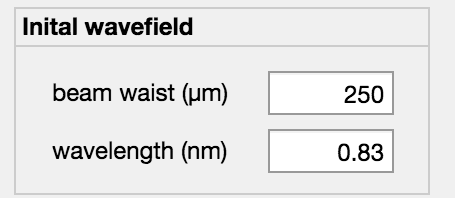
The initial wave field is given by a Gaussian beam defined by the beam part (1/e^2) and the wavelength. Both must be expressed in um.
In a future release it will also be possible to define any arbitrary input wave field. Both the amplitude and the phase must then be defined in a tiff file.
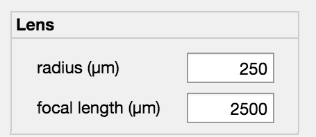
The (ideal) lens is defined by the aperture radius and focal length. Both must be specified in um.
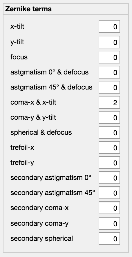
The Zernike Terms are standardized to the wavelength. Information about the Zernike polynomial and aberrations can be found on the website of James C. Wyant from the University of Arizona.
Link: wp.optics.arizona.edu/jcwyant/